💰 How to Build a Sensitivity Analysis That Shows Which Assumptions Affect Profit the Most

A forecast can look precise right up until one assumption changes. A modest shift in selling price, payroll, material costs, or customer volume can turn a promising profit plan into a difficult operating year.

That does not mean forecasting is pointless. It means a forecast should be treated as a model of uncertainty, not a promise about the future. Leaders need to know not only the expected profit, but also what could move it most.

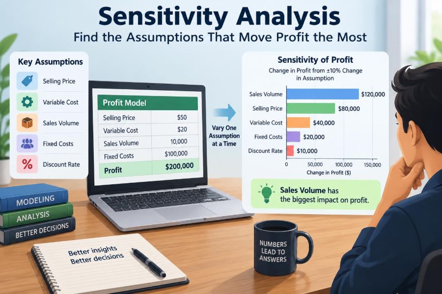
Sensitivity analysis answers that question. It tests how profit changes when one input changes while the other assumptions remain fixed, making the model’s pressure points visible.

For accounting students, it turns formulas into decision tools. For working professionals, it helps direct management attention toward the assumptions worth monitoring, negotiating, or validating before resources are committed.

🧭 Start With the Decision, Not the Spreadsheet

A useful sensitivity analysis begins with a real decision. You might be assessing a new product, preparing a budget, reviewing a capital investment, setting a price, or deciding whether an expansion plan is affordable.

The decision determines the right output. A pricing decision may focus on operating profit per month. A multi-year project may focus on net present value, while a lending discussion may focus on cash flow or debt-service coverage.

Without a defined decision, analysts often test every available input. The result is a busy worksheet that does not help anyone choose an action.

🎯 Define the Profit Measure Clearly

“Profit” is not one universal number. Gross profit, contribution margin, EBITDA, operating profit, earnings before tax, and net income each include different costs and can react differently to an assumption.

Choose the measure that matches the decision and label it clearly. If managers control prices and operating costs but not financing or tax policy, operating profit may be more useful than net income.

For a simple operating model:

Operating profit = Revenue − Variable costs − Fixed operating costs

Keep the definition consistent throughout the analysis. A comparison loses meaning if one case includes a cost that another excludes.

🧩 Build a Transparent Base Case

The base case is the central set of assumptions from which every sensitivity test starts. It should represent the planning case or best current estimate, not automatically the most optimistic outcome.

Use a model that another person can trace from assumptions to revenue, costs, and profit. Separate input cells from calculations and outputs rather than burying assumptions inside long formulas.

A transparent base case makes review faster and prevents a common error: changing an input that does not actually feed the reported profit figure.

🔗 Map the Economic Drivers of Profit

Before testing variables, map how the business makes and loses money. Revenue commonly depends on units sold, price, mix, returns, and timing. Costs may depend on volume, wages, supplier prices, capacity, commissions, exchange rates, or fixed commitments.

This map should reflect economic cause and effect, not merely the layout of the general ledger. “Cost of sales” is an accounting total; unit material cost, freight per shipment, and sales volume are more actionable drivers.

Ask a practical question: if this assumption changed in real life, which formula lines would move, and why?

📌 Select Assumptions That Are Both Uncertain and Material

Not every model input deserves equal attention. Prioritize assumptions that are uncertain, capable of changing profit materially, and relevant to management action.

Sales volume or utilization
Average selling price and discount rate
Variable cost per unit, including materials and shipping
Payroll rates, staffing levels, or overtime
Customer churn, returns, or bad-debt rates
Foreign exchange rates or commodity prices when exposure is significant

A highly uncertain but tiny office-supply expense may not matter. A stable but very large annual lease cost may deserve scenario treatment even if it is not a frequent sensitivity input.

🧱 Distinguish Inputs From Calculated Values

An input is an assumption you set, such as units sold or material cost per unit. A calculated value is produced by the model, such as total material cost or contribution margin.

Testing calculated values can conceal the business logic. If total variable cost is changed directly, the analysis may miss how volume, waste, supplier pricing, and product mix create that total.

Drive the model from the lowest practical level of controllable assumptions. That makes the result easier to explain and more useful when management asks what action could reduce the downside.

🧮 Use a Simple Profit Model Before Adding Complexity

A sensitivity analysis does not require an elaborate financial model. A simple hypothetical example is enough to show the method:

Units sold: 10,000
Selling price: $50 per unit
Variable cost: $30 per unit
Fixed costs: $150,000

Profit = (10,000 × ($50 − $30)) − $150,000 = $50,000

This structure reveals the drivers immediately. Higher units or price increase contribution; higher variable cost reduces it; fixed costs reduce profit dollar for dollar within the relevant range.

More detail should be added only where it improves the decision, such as tiered commissions, capacity constraints, taxes, or working-capital effects.

🔍 Understand One-Way Sensitivity Analysis

A one-way sensitivity analysis changes one assumption at a time while holding all others at their base-case values. It answers: “If this specific input is wrong, how much does profit change?”

For example, test sales volume at 9,000, 10,000, and 11,000 units while price, unit cost, and fixed costs remain unchanged. This isolates volume’s effect rather than mixing it with other causes.

One-way analysis is usually the best starting point because its results are direct, comparable, and easy to audit.

↔️ Choose Ranges That Reflect Real Possibilities

The range selected for each assumption has a major effect on the ranking. A wide price range and a narrow labor-cost range can make price appear dominant even when the ranges are not equally plausible.

Ranges should come from credible planning evidence where available: past variation, contracts, supplier quotations, pipeline data, capacity limits, known market conditions, or informed operational judgment.

When evidence is limited, state that the range is a planning assumption. Avoid presenting a convenient plus-or-minus percentage as if it were a measured probability distribution.

⚖️ Compare Consistent Change Bases

Inputs have different units. Selling price may be in dollars, volume in units, and wage cost in hourly rates. Comparing a $1 movement in each would be misleading.

Use a consistent basis, such as a defined low and high case, a percentage movement, or an operationally meaningful change. For a restaurant, 20 fewer customers per day may be more useful than a generic 5% demand reduction.

Consistency does not require identical percentages. It requires ranges that are defensible and clearly documented.

📊 Calculate the Effect on Profit

For each tested value, recalculate the model and record the output. The core measure is usually the change from base-case profit:

Profit effect = Profit under tested assumption − Base-case profit

In the hypothetical example, a $1 increase in unit variable cost lowers profit by $10,000 at 10,000 units. A $1 increase in selling price raises profit by the same amount, assuming volume does not change.

That last assumption matters. In real markets, price changes may affect demand, so a more realistic model may link price and volume rather than treating them as independent.

📏 Measure Downside, Upside, and Total Range

Do not report only one number when an assumption has both a low and high case. Separate downside from upside because management usually needs to understand the exposure as well as the opportunity.

Assumption	Low-case profit effect	High-case profit effect	What it reveals
Sales volume	Lower contribution	Higher contribution	Demand exposure
Selling price	Lower revenue per unit	Higher revenue per unit	Pricing power and discount risk
Variable cost per unit	Higher cost if input rises	Lower cost if input falls	Supplier and efficiency exposure

Total range, calculated as high-case profit minus low-case profit, is useful for ranking. Still, a single severe downside may deserve attention even when the total range is not the largest.

🌪️ Build a Tornado Chart for Fast Ranking

A tornado chart is a horizontal bar chart that ranks assumptions by their effect on the chosen output. The widest bars are placed at the top, producing the chart’s familiar tornado shape.

Each bar usually extends from the low-case profit result to the high-case profit result, with the base case marked at the center. It gives executives a fast answer to the question: which variables deserve discussion first?

The chart is not the analysis itself. It is a visual summary of tested assumptions, selected ranges, and model logic that must still be available for review.

🏷️ Label Charts So They Cannot Mislead

A chart should identify the output, currency, period, base case, and tested range. “Profit sensitivity” is vague; “FY budget operating profit sensitivity, base case $50,000” is clearer.

Label assumptions with both the driver and the range, such as “Unit sales: 9,000 to 11,000” or “Material cost: $28 to $33 per unit.” Readers should not have to search elsewhere to understand what each bar represents.

Use the same direction convention throughout. If the left side shows lower profit and the right side shows higher profit, preserve that arrangement for every driver.

🧠 Interpret Sensitivity as Exposure, Not Certainty

The biggest bar does not mean that outcome is most likely. It means profit changes the most across the range chosen for that assumption.

A supplier cost may have a large sensitivity but a low chance of moving because the company has a fixed-price contract. A smaller volume sensitivity may be more urgent if the sales pipeline is weak and the planning period is near.

Consider both impact and likelihood. Sensitivity analysis measures the first; a separate risk assessment is needed to judge the second.

🔄 Recognize When Drivers Are Connected

One-way sensitivity holds everything else constant, which is useful for isolation but can be unrealistic. Price reductions may increase volume. Lower volume may reduce purchasing discounts. Inflation may raise prices, wages, and materials together.

These relationships are called correlations or dependencies. Ignoring them can understate or overstate the combined exposure, especially when several drivers tend to worsen at the same time.

Document known connections rather than pretending they do not exist. Then use scenarios or two-way analysis to examine the most consequential combinations.

🗺️ Use Two-Way Sensitivity for Linked Decisions

A two-way sensitivity analysis changes two inputs simultaneously. It is particularly useful when management controls one variable but faces uncertainty in another.

For example, a price-volume table can show profit across several selling prices and unit-sales levels. The table helps answer questions such as: how many additional units must be sold to offset a $2 price reduction?

Keep the number of dimensions limited. A three- or four-variable grid quickly becomes difficult to read and can hide the main message.

🎬 Build Scenarios for Coherent Business Stories

Scenarios change several assumptions in a way that reflects a plausible operating story. A downside scenario might combine weaker demand, more discounting, and higher freight costs if those conditions could occur together.

Unlike one-way sensitivity, scenarios do not isolate a single driver. Their purpose is to show the effect of a connected set of conditions on profit, cash flow, capacity, and covenant headroom.

🧾 A practical scenario set

Base case: current planning assumptions.
Upside case: favorable but credible conditions, not wishful inputs.
Downside case: adverse conditions that management should be prepared to manage.

Use sensitivity analysis to identify key drivers, then use scenarios to tell the wider operational story.

💵 Separate Profit Sensitivity From Cash Sensitivity

Profit and cash are related but not identical. A sales increase can improve accounting profit while consuming cash through inventory, receivables, additional production, or delayed customer collection.

Likewise, depreciation reduces profit but does not create a current-period cash payment. A capital expenditure may reduce cash immediately while affecting profit gradually through depreciation.

If the decision concerns liquidity, debt capacity, or survival through a weak period, build a parallel cash-flow sensitivity analysis. Do not assume the profit tornado chart answers a cash question.

🏭 Respect Fixed Costs, Capacity, and Step Changes

Simple models often assume costs behave smoothly. Real businesses frequently have thresholds: a new shift, warehouse, machine, supervisor, or delivery vehicle may be needed after volume reaches a certain level.

These are step costs. Profit may rise with volume until capacity is reached, then drop or flatten when an additional fixed commitment becomes necessary.

Model capacity limits explicitly when they matter. Otherwise, high-volume cases can imply margins that are impossible to achieve with available people, space, or equipment.

📈 Watch for Nonlinear Relationships

A driver’s effect is not always constant. Tiered supplier pricing, progressive commissions, volume rebates, overtime premiums, and tax thresholds can create nonlinear results.

In those cases, testing only a small movement around the base case may hide a significant change farther away. Use several test points and inspect the profit curve rather than assuming a straight line.

Nonlinearity is not a reason to abandon sensitivity analysis. It is a reason to make the model reflect the actual terms and operating constraints.

🧾 Document Sources, Ownership, and Timing

Every key assumption should have a short record: definition, base value, tested range, source or rationale, owner, and date last reviewed. This turns a one-time workbook into a controllable planning process.

For example, the procurement team may own material-cost assumptions, sales leadership may own volume and discount assumptions, and operations may own labor productivity. Finance coordinates the model but should not silently invent operational inputs.

Assumption ownership improves accountability because the people closest to the driver can challenge stale or unsupported values.

🛠️ Set Up the Spreadsheet for Auditability

In a spreadsheet, place assumptions in a clearly marked input area and keep calculations in separate sections. Use consistent units and time periods; a monthly price should not accidentally feed an annual volume formula.

Useful controls include:

Checks that revenue equals units multiplied by price.
Flags for negative volumes, implausible margins, or missing assumptions.
Named input ranges or clear cell labels.
A version date and a record of material changes.

Spreadsheet data tables can automate one- and two-way tests, but manual recalculation is often easier to audit in a smaller model. Choose the method the team can maintain reliably.

🚫 Avoid the Most Common Modeling Errors

A frequent mistake is changing several inputs at once and calling the result a sensitivity. That is a scenario, and it should be labeled as one. Another is mixing monthly and annual figures, which can make a result look credible while being wrong by a large factor.

Other avoidable errors include hard-coded overrides, double-counted cost changes, circular references, and formulas that fail to update when a test value changes. Formula auditing and a few hand calculations are essential safeguards.

Also avoid false precision. Reporting profit sensitivity to the nearest dollar may imply a reliability that the underlying assumptions do not support.

🧯 Do Not Confuse Risk Ranking With Management Action

A tornado chart ranks exposures; it does not automatically prescribe action. The largest driver may be difficult or costly to control, while a smaller driver may be manageable through a concrete operational change.

For each major sensitivity, ask three questions:

Can we influence this driver?
What early indicator would warn us that it is moving?
What response can reduce the downside or capture the upside?

For instance, a material-cost sensitivity may lead to supplier negotiations, alternate sourcing, hedging where appropriate, product redesign, or revised pricing. The right response depends on the business, contracts, and timing.

🚦Turn Results Into Monitoring Triggers

The analysis becomes valuable when it changes routine management behavior. Convert important assumptions into measurable indicators such as order intake, conversion rates, average discount, scrap rate, labor hours per unit, or supplier quotations.

Define trigger points in advance. If weekly orders fall below the rate needed to support the budget, management can revise production plans, spending, or sales activity before a month-end surprise.

Triggers are not predictions. They are decision rules that connect model insight to timely review.

🤝 Present the Findings for the Audience

Executives may need one chart, three risks, and recommended actions. Operating managers may need detailed driver definitions and weekly indicators. Analysts need formulas, source data, and reconciliation checks.

Adapt the presentation without changing the underlying model. A concise summary should still state the base profit, time period, key tested ranges, and important limitations.

A good presentation invites challenge. If a leader asks why volume is ranked above price, the analysis should make the ranges and contribution mechanics easy to explain.

🧪 Review the Model Against Actual Results

A sensitivity model should improve over time. Compare actual volume, pricing, costs, and profit with the assumptions used in the forecast. Identify whether differences came from an incorrect range, an omitted driver, timing, or execution.

This is not about blaming the original forecast. It is about learning which assumptions are consistently uncertain and where the business model needs more detail.

Regular review also prevents outdated conditions, such as expired supplier contracts or changed staffing plans, from remaining embedded in the planning case.

🪜 A Repeatable Workflow

Define the decision, period, and profit measure.
Build and check a transparent base-case model.
Identify uncertain, material economic drivers.
Set documented low and high ranges for each driver.
Run one-way tests and calculate profit changes.
Rank results in a tornado chart.
Test linked drivers with two-way tables or scenarios.
Assign owners, indicators, and response actions.
Refresh the analysis as actual results and conditions change.

This workflow is deliberately simple. Its discipline matters more than sophisticated formatting.

🏁 The Core Principle: Make Assumptions Visible and Actionable

The purpose of sensitivity analysis is not to create a dramatic chart or claim that the future has been calculated. Its purpose is to expose where a profit plan is most vulnerable and where management attention can make the greatest difference.

Start with a clear profit definition, test realistic ranges one driver at a time, and distinguish isolated sensitivities from connected scenarios. Then translate the largest exposures into monitoring and action.

When the model is transparent, ranges are defensible, and results are interpreted with appropriate caution, sensitivity analysis becomes a practical bridge between accounting information and better business decisions.

The best sensitivity analysis does not predict every outcome; it shows which assumptions deserve to be understood, watched, and managed first. 💰📊🧭